

In 2020, I got an interesting email in my inbox from another mollusk researcher! Niels de Winter had emailed me, who I was familiar with from his past work on big Cretaceous rudist bivalves and giant snails. Niels had seen my paper published that year on giant clam shell isotopes from the Gulf of Aqaba in the Northern Red Sea, and was interested in teaming up on a new study to compare the daily growth of giant clams with another bivalve that has daily growth: scallops! I was intrigued because I had similar work underway to study the shells of clams I was growing at Biosphere 2, but I didn’t have any plans to measure my collected wild clam shells that way. So this sounded like a win-win opportunity to work together on a study that neither of us could do alone! Plus, I liked his work and had cited it in the past.
The shells of bivalves are very useful as each produces a shell diary consisting of growth lines, similar to the rings of a tree. Giant clams keep a very detailed diary, with a new growth line forming every night, which previous research has suggested was due to the control that the symbiotic algae inside giant clams have on their host. When the algae conduct photosynthesis, they use CO₂ in the fluid the clam makes its shell from, which increases the pH and accelerates the formation of the shell mineral crystals! The symbionts also directly assist by pumping calcium and other raw materials for the clam to use! Niels had found such daily lines in an ancient rudist bivalve from over 66 million years ago, and proposed it as a sign that the rudists might have had similar algae! I used the daily lines to compare giant clam growth before and after humans arrived in the Red Sea, finding that the clams are growing faster!
But it turns out that giant clams aren’t the only bivalves that make daily lines. Some species of scallops do it too, but that’s a bit confusing, since scallops have no symbionts that could be producing this daily growth period! One way we could investigate this is by bombarding the shells with very tiny laser beams only 20 µm across: the width of a hair is a flawed unit of measurement but 20 microns is as narrow as the narrowest type of hair you can think of! The laser would carry across the cross sections of the shell in a line, literally burning away tiny bits of shell, with the resulting gases captured by a machine called a mass spectrometer, which can figure out the concentrations of elements in the gas.
So we’d basically create a very detailed wiggly graph, where the wiggles represent years, months, days and even tides, depending on how fast the clams and scallops grew! I’m happy to report the paper was published earlier this year, so I thought I’d switch it up a bit and have a conversation with Niels through this blog post. Let me open it up to Niels, who I decided to bring in for this post in a kind of conversation!
Niels, what did you expect to find heading into this experiment? For me, I figured the giant clams would have greater amplitude of variation on a daily basis than the scallops, due to the influence of the symbionts. Is this what you expected?
More or less. To be honest, that is what I was hoping to find, because if the daily lines were so much stronger in photosymbiotic shells than in the non-photosymbiotic scallops, it would make it easier to recognize photosymbiosis by studying modern and fossil shells. Also, a finding like that would obviously support the hypothesis we had about the ancient rudist bivalve. However, I was a bit skeptical as to whether the reality would be so clear-cut.
I mailed samples from six juvenile giant clams to Niels for analysis. We went with juveniles for a couple reasons: they grow faster at this life stage than they do as adults: 2-5 centimeters per year for the species we were studying, which meant the greatest opportunity to record a very detailed record from their shells! Scallops also grow extremely quickly, up to 5 cm/year, and so we would be able to get a similar resolution for both types of bivalves, since each page in their diaries would be a similar width.
Niels brought in our collauthors Lukas Fröhlich, a scallop expert, as well as other geochemists like Lennart de Nooijer, Wim Boer, Bernd Schöne, Julien Thébault, and Gert-Jan Reichart. Could you tell us about the other members of the team and how you brought them in?
When I start a new study like this, I always like to “outsource” the expertise about the topic a bit. Our work in sclerochronology often involves bringing together several fields of research and interpreting the results of complex measurements like these requires input from several people who look at them from different viewpoints. I had just finished a research stay at the University of Mainz in 2019, where I worked with Bernd Schöne and Lukas Fröhlich. I know Lukas was working on scallops together with Julien Thébault, whose team collects them alive in the Bay of Brest and keeps a very detailed record of the circumstances the scallops grow at. To carry out the laser measurements, I needed geochemistry experts, and Lennart de Nooijer, Wim Boer and Gert-Jan Reichart came to mind because I was already working with them on other topics and they run a very good lab for these analyses at the Royal Netherlands Institute for Sea Research (NIOZ). This is how the team came together.
Niels conducted a series of laser transects across the clam shells. He used some sophisticated time series analysis approaches to try to quantify the different periodic cycles that appeared in the clam and scallop growth. This was a different approach to how other workers have gone about finding daily growth cycles in giant clams and scallops, where they have often started by zooming in to find the wiggles, and work backwards from there. Niels instead tried to agnostically dissemble the growth records across each clam shell using mathematical approaches, based on the idea that this would be how future workers have to go about identifying daily growth patterns in fossil clams, where we often don’t have a real “growth model” up front to work with. By growth model, I mean the way that we convert the geochemical observations, which are arranged by distance along the shell, into units of time, which requires us to know how fast the clams grew. For the scallops, the age model was made by counting daily “striae” they form on the outside of their shells. For the giant clams, I helped with this by counting tiny growth lines inside the shell made visible by applying a dye called Mutvei’s solution. Because the growth lines weren’t visible all the way through the shell, I used a von Bertalanffy model to bridge across and create a continuous estimate of how old the clams were at each point along their shells.
Niels found some interesting results! I personally expected that the daily variation in giant clams would dwarf what was seen in the scallops, because of the impact of the daily activity of the symbionts. But it turned out that while the clams had a more regular pattern of daily shell growth than the scallops, likely controlled by the symbionts, that was still a minority of the variance across the clams’ records. Yet again, these clams destroyed my hypothesis, but in an interesting way!
Niels, what were your expectations going into this, and how did the results confirm or go against your hypotheses? What challenges did you run into in the course of your analysis, and how did you end up addressing those challenges?
This was honestly one of the most difficult shell-datasets I have worked with so far. The laser technique we used measures the elemental composition of the shells in very high detail, but while this is ideal for funding daily rhythms, it is both a blessing and a curse! In a dataset like this it becomes quite hard to separate the signal we are interested in from the noise that occurs due to measurement uncertainty. I ended up using a technique called spectral analysis, which is often used to detect rhythmic changes in successions of rocks. I guess this is where my geology background was helpful. With this technique, we were able to “filter out” the variability in the records of shell composition that happened at the scale of days and tides and remove the noise and the longer timescale variations. It turns out that, when you do this, you have to remove a surprisingly large fraction of the data, which shows us that the influence of the daily cycle on the composition of both the scallops and the clams is not very large (at most 20%). We did find a larger contribution in the giant clams, as expected, but the difference was much smaller than anticipated. I also find it interesting that most of the variability was not rhythmic. This shows that there are likely processes at play that control the composition of shells on a daily basis which we do not understand yet.
We were measuring a suite of different elements across both bivalve species, including strontium, magnesium, manganese and barium. All of these were reported relative to calcium, the dominant metal ion in the shell material (they’re made of calcium carbonate). This is why we call them “trace” elements; each is integrated into the material of the shell due to a variety of causes, including the temperature, the composition of the seawater, the growth rate of the clams, and also simply due to chance.
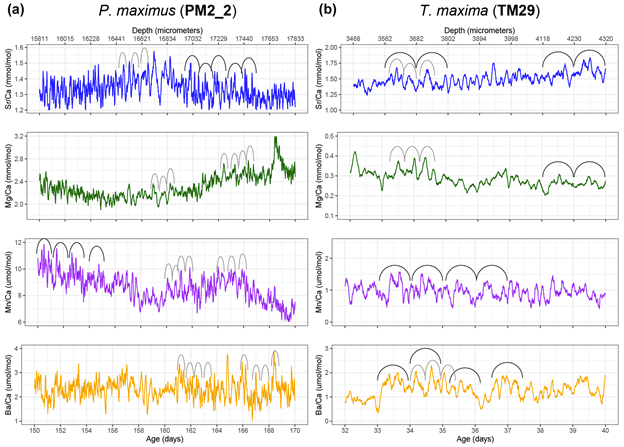
In the giant clams, the elements that varied most on a daily basis were strontium and barium. Prior workers had found strontium was the strongest in terms of daily variation, but barium was more unexpected! Normally, barium is thought of as a record of the activity of plankton in the environment, and since there is very little plankton to be found in the Red Sea, it was not expected to see that element vary on a daily basis. It could be that barium gets included in the shell more as a function of the growth rate of the animals. Meanwhile, the scallops (from the Bay of Brest in France) were measuring strong tidal variability in barium and strontium, which makes sense because that location has huge tides compared to the Red Sea. Tides happen on periods of ~12.4 and 24.8 hours. The scallops showed swings lining up with both, and the tidal variability might be the main explanation for how scallops form daily lines. Because the lunar day is so close to a solar day, they would be hard to tell apart from each other! Interestingly, the giant clams also showed some sign of a ~12 hour cycle. While the Red Sea has pretty tiny tides, I had noticed that some of the clams make 2 growth lines a day, and if some clams in the shallowest waters were exposed on a tidal basis, that could explain why they’d make 2 lines: one at low tide, and one at night! Even in places without tides, like the Biosphere 2 ocean, I’d noticed evidence of 12-hour patterns of activity in the clams. It’s so nice (and rare!) when one of my hypotheses is confirmed!
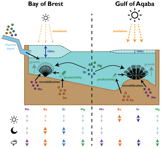
Both the giant clams and scallops recorded large irregular swings in all of the studied elements, likely due to non-periodic disturbances. In the case of the scallops, these included storms and the floods of sediment from rivers. For the giant clams, these probably included algae blooms that affect the Red Sea, as well as potentially dust storms that also come every 1-2 years. Both giant clams and scallops have a lot of potential to measure paleo-weather, which is something that other researchers have observed as well!
Niels, where do you see this work heading next?
The recent work looking at very short-term changes in shells is very promising, I think. I agree that there might be a possibility to detect weather patterns in these shells, but that would require some more work into understanding how these animals respond to changes in their environment on an hourly scale and what that response does to their shell composition.
In the meantime, I was intrigued to find that we were not the only people looking for daily cycles in the chemistry of giant clam shells. I had the pleasure of reviewing this paper by Iris Arndt and her colleagues from the university of Frankfurt (Germany). Iris took a similar approach to detecting these daily cycles by using spectral analysis, but she a smart tool called a “wavelet analysis” to visualize the presence of daily rhythms in the shell, which I think was more successful than my approach. She even wrote a small piece of software which can be used to (almost) automatically detect the days and “date” the clam shell based on them. This is quite a step forward, and if I were to do a project like this again, I would certainly try our Iris’ method.
Interesting, too, is that the fossil giant clams studied by Iris showed the daily cycles in magnesium concentration instead of strontium and barium. This shows that the incorporation of trace metals into clam shells is still not fully understood. So one of the things to do, in my opinion, would be to try to see if we can use shells grown under controlled conditions to link the shell composition to short-term changes in the environment. This would require a complex experimental setup in which we simulate an artificial day and night rhythm or an artificial “storm”, but I think it can be done using the culture experiments we do at the NIOZ.
This study represented a unique opportunity to collaborate with my colleague Niels on a topic that interested both of us, which we wouldn’t have been able to pursue on our own. I enjoyed collaborating with him on this work and we have some ideas for further studies down the road, so stay tuned for the next co-clam-boration!

